neuro models

• introduction
  • overview
  • historical ai
  • historical cybernetics/nns
• neuron models
  • circuit-modelling basics
  • action potentials
  • physics of computation
• supervised learning
• unsupervised learning
  • hebbian learning and pca
• sparse, distributed coding
• self-organizing maps
• recurrent networks
• probabilistic models + inference
• boltzmann machines
• ica
• spiking neurons
• high-dimensional computing
  • definitions
  • ex. identify the language
  • mathematical background
  • comparison to DNNs
  • different names
  • theory of sequence indexing and working memory in RNNs

---

• convs are organized spatially
• could do transform so that have spatial convs that are organized spatially, orientation based, frequency based

introduction

overview

• does biology have a cutoff level (likecutoffs in computers below which fluctuations don’t matter)
• core principles underlying these two questions
  • how do brains work?
  • how do you build an intelligent machine?
• lacking: insight from neuro that can help build machine
• scales: cortex, column, neuron, synapses
• physics: theory and practice are much closer
• are there principles?
  • “god is a hacker” - francis crick
  • theorists are lazy - ramon y cajal
  • things seemed like mush but became more clear - horace barlow
  • principles of neural design book
• felleman & van essen 1991
  • ascending layers (e.g. v1-> v2): goes from superficial to deep layers
  • descending layers (e.g. v2 -> v1): deep layers to superficial
• solari & stoner 2011 “cognitive consilience” - layers thicknesses change in different parts of the brain
  • motor cortex has much smaller input (layer 4), since it is mostly output

historical ai

• people: turing, von neumman, marvin minsky, mccarthy…
• ai: birth at 1956 conference
  • vision: marvin minsky thought it would be a summer project
• lighthill debate 1973 - was ai worth funding?
• intelligence tends to be developed by young children…
• cortex grew very rapidly

historical cybernetics/nns

• people: norbert weiner, mcculloch & pitts, rosenblatt
• neuro
  • hubel & weisel (1962, 1965) simple, complex, hypercomplex cells
  • neocognitron fukushima 1980
  • david marr: theory, representation, implementation

neuron models

circuit-modelling basics

• membrane has capacitance $C_m$
• force for diffusion, force for drift
• can write down diffeq for this, which yields an equilibrium
• $\tau = RC$
  • bigger $\tau$ is slower
  • to increase capacitance
    • could have larger diameter
    • $C_m \propto D$
  • axial resistance $R_A \propto 1/D^2$ (not same as membrane lerk), thus bigger axons actually charge faster

action potentials

• channel/receptor types
  • ionotropic: $G_{ion}$ = f(molecules outside)
    • something binds and opens channel
  • metabotropic: $G_{ion}$ = f(molecules inside)
    • doesn’t directly open a channel: indirect
  • others
    • photoreceptor
    • hair cell
  • voltage-gated (active - provide gain; might not require active ATP, other channels are all passive)

physics of computation

• based on carver mead: drift and diffusion are at the heart of everything
• different things realted by the Boltzmann distr. (ex. distr of air molecules vs elevation. Subject to gravity and diffusion upwards since they’re colliding)
  • nernst potential
  • current-voltage relation of voltage-gated channels
  • current-voltage relation of MOS transistor
• these things are all like transistor: energy barrier that must be overcome
• neuromorphic examples
  • differential pair sigmoid yields sigmoid-like function
    • can compute tanh function really simply to simulate
  • silicon retina
    • lateral inhibition exists (gap junctions in horizontal cells)
    • mead & mahowald 1989 - analog VLSI retina (center-surround receptive field is very low energy)
• computation requires energy (otherwise signals would dissipate)
  • von neumann architecture: CPU - bus (data / address) - Memory
    • moore’s law ending (in terms of cost, clock speed, etc.)
      • ex. errors increase as device size decreases (and can’t tolerate any errors)
  • neuromorphic computing
    • brain ~ 20 Watts
    • exploit intrinsic transistor physics (need extremely small amounts of current)
    • exploit electronics laws kirchoff’s law, ohm’s law
    • new materials (ex. memristor - 3d crossbar array)
    • can’t just do biological mimicry - need to understand the principles

supervised learning

• see machine learning course
• net talk was major breakthrough (words -> audio) Sejnowski & Rosenberg 1987
• people looked for world-centric receptive fields (so neurons responded to things not relative to retina but relative to body) but didn’t find them
  • however, they did find gain fields: (Zipser & Anderson, 1987)
    • gain changes based on what retina is pointing at
  • trained nn to go from pixels to head-centered coordinate frame
    • yielded gain fields
  • pouget et al. were able to find that this helped having 2 pop vectors: one for retina, one for eye, then add to account for it
• support vector networks (vapnik et al.) - svms early inspired from nns
• dendritic nonlinearities (hausser & mel 03)
• example to think about neurons due this: $u = w_1 x_1 + w_2x_2 + w_{12}x_1x_2$
  • $y=\sigma(u)$
  • somestimes called sigma-pi unit since it’s a sum of products
  • exponential number of params…could be fixed w/ kernel trick?
    • could also incorporate geometry constraint…

unsupervised learning

• born w/ extremely strong priors on weights in different areas
• barlow 1961, attneave 1954: efficient coding hypothesis = redundancy reduction hypothesis
  • representation: compression / usefulness
  • easier to store prior probabilities (because inputs are independent)
  • relich 93: redundancy reduction for unsupervised learning (text ex. learns words from text w/out spaces)

hebbian learning and pca

• pca can also be thought of as a tool for decorrelation (in pc dimension, tends to be less correlated)
• hebbian learning = fire together, wire together: $\Delta w_{ab} \propto <a, b>$ note: $<a, b>$ is correlation of a and b (average over time)
• linear hebbian learning (perceptron with linear output)
• $\dot{w}_i \propto <y, x_i> \propto \sum_j w_j <x_j, x_i>$ since weights change relatively slowly
  • synapse couldn’t do this, would grow too large
• oja’s rule (hebbian learning w/ weight decay so ws don’t get too big)
  • points to correct direction
• sanger’s rule: for multiple neurons, fit residuals of other neurons
• competitive learning rule: winner take all
  • population nonlinearity is a max
  • gets stuck in local minima (basically k-means)
• pca only really good when data is gaussian
  • interesting problems are non-gaussian, non-linear, non-convex
• pca: yields checkerboards that get increasingly complex (because images are smooth, can describe with smaller checkerboards)
  • this is what jpeg does
  • very similar to discrete cosine transform (DCT)
  • very hard for neurons to get receptive fields that look like this
• retina: does whitening (yields center-surround receptive fields)
  • easier to build
  • gets more even outputs
  • only has ~1.5 million fibers

sparse, distributed coding

• \[\underset {\mathbf{D}} \min \underset t \sum \underset {\mathbf{h^{(t)}}} \min ||\mathbf{x^{(t)}} - \mathbf{Dh^{(t)}}||_2^2 + \lambda ||\mathbf{h^{(t)}}||_1\]
  • D is like autoencoder output weight matrix
  • h is more complicated - requires solving inner minimization problem
  • outer loop is not quite lasso - weights are not what is penalized
• barlow 1972: want to represent stimulus with minimum active neurons
  • neurons farther in cortex are more silent
  • v1 is highly overcomplete (dimensionality expansion)
• codes: dense -> sparse, distributed $n \choose k$ -> local (grandmother cells)
  • energy argument - bruno doesn’t think it’s a big deal (could just not have a brain)
• PCA: autoencoder when you enforce weights to be orthonormal
  • retina must output encoded inputs as spikes, lower dimension -> uses whitening
• cortex
  • sparse coding different kind of autencoder bottleneck (imposes sparsity)
• using bottlenecks in autoencoders forces you to find structure in data
• v1 simple-cell receptive fields are localized, oriented, and bandpass
• higher-order image statistics
  • phase alignment
  • orientation (requires at least 3 points stats (like orientation)
  • motion
• how to learn sparse repr?
  • foldiak 1990 forming sparse reprs by local anti-hebbian learning
  • driven by inputs and gets lateral inhibition and sum threshold
  • neurons drift towards some firing rate naturally (adjust threshold naturally)
• use higher-order statistics
  • projection pursuit (field 1994) - maximize non-gaussianity of projections
    • CLT says random projections should look gaussian
    • gabor-filter response histogram over natural images look non-Gaussian (sparse) - peaked at 0
  • doesn’t work for graded signals
• sparse coding for graded signals: olshausen & field, 1996
  • $\underset{Image}{I(x, y)} = \sum_i a_i \phi_i (x, y) + \epsilon (x,y)$

  • loss function $\frac{1}{2}

    I - \phi a

    ^2 + \lambda \sum_i C(a_i)$

  • can think about difference between $L_1$ and $L_2$ as having preferred directions (for the same length of vector) - prefer directions which some zeros
  • in terms of optimization, smooth near zero
  • there is a network implementation
  • $a_i$are calculated by solvin optimization for each image, $\phi$ is learned more slowly
  • can you get $a_i$ closed form soln?
• wavelets invented in 1980s/1990s for sparsity + compression
• these tuning curves match those of real v1 neurons
• applications
  • for time, have spatiotemporal basis where local wavelet moves
  • sparse coding of natural sounds
    • audition like a movie with two pixels (each ear sounds independent)
    • converges to gamma tone functions, which is what auditory fibers look like
  • sparse coding to neural recordings - finds spikes in neurons
    • learns that different layers activate together, different frequencies come out
    • found place cell bases for LFP in hippocampus
  • nonnegative matrix factorization - like sparse coding but enforces nonnegative
  • can explicitly enforce nonnegativity
• LCA algorithm lets us implement sparse coding in biologically plausible local manner
• explaining away - neural responses at the population should be decodable (shouldn’t be ambiguous)
• good project: understanding properties of sparse coding bases

• SNR = $VAR(I) / VAR(

  I- \phi A

  )$

• can run on data after whitening
  • graph is of power vs frequency (images go down as $1/f$), need to weighten with f
  • don’t whiten highest frequencies (because really just noise)
    • need to do this softly - roughly what the retina does
  • as a result higher spatial frequency activations have less variance
• whitening effect on sparse coding
  • if you don’t whiten, have some directions that have much more variance
• projects
  • applying to different types of data (ex. auditory)
• adding more bases as time goes on
• combining convolution w/ sparse coding?
• people didn’t see sparsity for a while because they were using very specific stimuli and specific neurons
  • now people with less biased sampling are finding more sparsity
  • in cortex anasthesia tends to lower firing rates, but opposite in hippocampus

self-organizing maps

• homunculus - 3d map corresponds to map in cortex (sensory + motor)
• visual cortex
  • visual cortex mostly devoted to center
  • different neurons in same regions sensitive to different orientations (changing smoothly)
  • orientation constant along column
  • orientation maps not found in mice (but in cats, monkeys)
  • direction selective cells as well
• maps are plastic - cortex devoted to particular tasks expands (not passive, needs to be active)
  • kids therapy with tone-tracking video games at higher and higher frequencies

recurrent networks

• hopfield nets can store / retrieve memories
• fully connected (no input/output) - activations are what matter
  • can memorize patterns - starting with noisy patterns can converge to these patterns
• marr-pogio stereo algorithm
• hopfield three-way connections
  • $E = - \sum_{i, j, k} T_{i, j, k} V_i V_j V_k$ (self connections set to 0)
    • update to $V_i$ is now bilinear
• dynamic routing
  • hinton 1981 - reference frames requires structured representations
    • mapping units vote for different orientations, sizes, positions based on basic units
    • mapping units gate the activity from other types of units - weight is dependent on if mapping is activated
    • top-down activations give info back to mapping units
    • this is a hopfield net with three-way connections (between input units, output units, mapping units)
    • reference frame is a key part of how we see - need to vote for transformations
  • olshausen, anderson, & van essen 1993 - dynamic routing circuits
    • ran simulations of such things (hinton said it was hard to get simulations to work)
    • we learn things in object-based reference frames
    • inputs -> outputs has weight matrix gated by control
  • zeiler & fergus 2013 - visualizing things at intermediate layers - deconv (by dynamic routing)
    • save indexes of max pooling (these would be the control neurons)
    • when you do deconv, assign max value to these indexes
  • arathom 02 - map-seeking circuits
  • tenenbaum & freeman 2000 - bilinear models
    • trying to separate content + style
  • hinton et al 2011 - transforming autoencoders - trained neural net to learn to shift imge
  • sabour et al 2017 - dynamic routing between capsules
    • units output a vector (represents info about reference frame)
    • matrix transforms reference frames between units
    • recurrent control units settle on some transformation to identify reference frame

probabilistic models + inference

Wiener filter

has Gaussian prior + likelihood

• gaussians are everywhere because of CLT, max entropy (subject to power constraint)

  • for gaussian function, $d/dx f(x) = -x f(x)$

boltzmann machines

• hinton & sejnowski 1983
• starts with a hopfield net (states $s_i$ weights $\lambda_{ij}$) where states are $\pm 1$
• define energy function $E(\mathbf{s}) = - \sum_{ij} \lambda_{ij} s_i s_j$
• assume Boltzmann distr $P(s) = \frac{1}{z} \exp (- \beta \phi(s))$
• learning rule is basically expectation over data - expectation over model
  • could use wake-sleep algorithm
  • during day, calculate expectation over data via Hebbian learning (in Hopfield net this would store minima)
  • during night, would run anit hebbian by doing random walk over network (in Hopfield ne this would remove spurious local minima)
• learn via gibs sampling (prob for one node conditioned on others is sigmoid)
• can add hiddent units to allow for learning higher-order interactions (not just pairwise)
  • restricted boltzmann machine: no connections between “visible” units and no connections between “hidden units”
  • computationally easier (sampling is independent) but less rich
• stacked rbm: hinton & salakhutdinov (hinton argues this is first paper to launch deep learning)
  • don’t train layers jointly
  • learn weights with rbms as encoder
  • then decoder is just transpose of weights
  • finally, run fine-tuning on autoencoder
  • able to separate units in hidden layer
  • cool - didn’t actually need decoder
• in rbm
  • when measuring true distr, don’t see hidden vals
    • instead observe visible units and conditionally sample over hidden units

    • $P(h

      v) = \prod_i P(h_i

      v)$ ~ easy to sample from

  • when measuring sampled distr., just sample $P(h

    v)$ then sample $P(v

    h)$

• ising model - only visible units
  • basically just replicates pairwise statistics (kind of like pca)
    • pairwise statistics basically say “when I’m on, are my neighbors on?”
  • need 3-point statistics to learn a line
• generating textures
  • learn the distribution of pixels in 3x3 patches
  • then maximize this distribution - can yield textures
• reducing the dimensionality of data with neural networks

ica

• PCA vs ICA: both have $X = As$, where $s$ is components (assume X has zero mean)
  • PCA / factor analysis assume $s$ Gaussian, want to decorrelate them
    • $\mathbb E [s_i \cdot s_j] = 0$
    • when Gaussian this implies independenct
  • ICA: assume s not Gaussian, want to make them independent
    • $P(s) = \prod_i P(s_i)$
    • this is a special case of sparse coding
• bell & sejnowski 1995
  • entropy maximization - try to find a nonlinear function $g(x)$ which lets you map that distr $f(x)$ to uniform
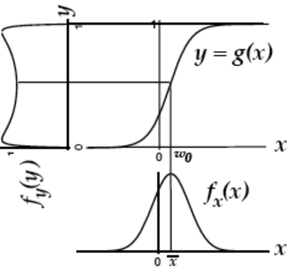
  • then, that function $g(x)$ is the cdf of $f(x)$
  • in ICA, we do this for higher dims - want to map distr of $x_1, …, x_p$ to $y_1, …, y_p$ where distr over $y_i$’s is uniform (implying that they are independent)
    • additionally we want the map to be information preserving

  • mathematically: $\underset{W} \max I(x; y) = \underset{W} \max H(y)$ since $H(y

    x)$ is zero (there is no randomness)

    • assume $y = \sigma (W x)$ where $\sigma$ is elementwise
    • (then S = WX, $W=A^{-1}$)

    • requires certain assumptions so that $p(y)$ is still a distr. :$p(y) = p(x) /

      J

      $ where J is Jacobian

  • learn W via gradient ascent $\Delta W \propto \partial / \partial W (\log

    J

    )$

    • there is now something faster called fast ICA
  • relationship to sparse coding
    • ICA can be a special case of sparse coding…
    • can think of cost as a prior over coefficients (Laplacian distr.) and reconstruction error as likelihood model
    • can write down posterior distr, derive learning on A for gradient ascent
  • topographic ICA (make nearby coefficient like each other)
• model predicts and all that’s passed on is the residual

spiking neurons

• passive membrane model was leaky integrator
• voltage-gaed channels were more complicated
• can be though of as leaky integrate-and-fire neuron (LIF)
  • this charges up and then fires a spike, has refractory period, then starts charging up again
• rate coding hypothesis - signal conveyed is the rate of spiking (bruno thinks this is usually too simple)
  • spiking irregulariy is largely due to noise and doesn’t convey information
  • some neurons (e.g. neurons in LIP) might actually just convey a rate
• linear-nonlinear-poisson model (LNP) - sometimes called GLM (generalized linear model)
  • based on observation that variance in firing rate $\propto$ mean firing rate
    • plotting mean vs variance = 1 $\implies$ Poisson output
  • these led people to model firing rates as Poisson $\frac {\lambda^n e^{-\lambda}} {n!}$
  • bruno doesn’t really believe the firing is random (just an effect of other things we can’t measure)
  • ex. fly H1 neuron 1997
    • constant stimulus looks very Poisson
    • moving stimulus looks very Bernoulli
• spike timing hypothesis
  • spiece timing can be very precise in response to time-varying signals (mainen & sejnowski 1995; bair & koch 1996)
  • often see precise timing
• encoding: stimulus $\to$ spikes
• decoding: spikes $\to$ representation
• encoding + decoding are related through the joint distr. over simulus and repsonse (see Bialek spikes book)
  • nonlinear encoding function can yield linear decoding
  • able to directly decode spikes using a kernel to reproduce signal (seems to say you need spikes - rates would not be good enough)
    • some reactions happen too fast to average spikes (e.g. 30 ms)
  • estimating information rate: bits (usually better than snr - can calculate between them) - usually 2-3 bits/spike

high-dimensional computing

• high-level overview
  • current inspiration has all come from single neurons at a time - hd computing is going past this
  • the brain’s circuits are high-dimensional
  • elements are stochastic not deterministic
  • can learn from experience
  • no 2 brains are alike yet they exhibit the same behavior
• basic question of comp neuro: what kind of computing can explain behavior produced by trains?
  • recognizing ppl by how they look, sound, or behave
  • learning from examples
  • remembering things going back to childhood
  • communicating with language

definitions

• what is hd computing
  • compute with random high-dim vectors
  • ex. 10k vectors A, B of +1/-1 (also extends to real / complex vectors)
• 3 operations
  • addition: A + B = (0, 0, 2, 0, 2,-2, 0, ….)
  • multiplication: A * B = (-1, -1, -1, 1, 1, -1, 1, …)
  • permutation: shuffles values
    • ex. rotate (bit shift with wrapping around)
• these operations allow for encoding all normal data structures: sets, sequences, lists, databases
• similarity = dot product (sometimes normalized)
  • A . A = 10k
  • A . A = 0 - orthogonal
  • in high-dim spaces, almost all pairs of vectors are dissimilar A. B = 0
  • goal similar meanings should have large similarity
• benefits - very simple and scalable - only go through data once
  • equally easy to use 4-grams vs. 5-grams

ex. identify the language

• data
  • train: given million bytes of text per language (in the same alphabet)
  • test: new sentences for each language
• training: compute a 10k profile vector for each language and for each test sentence
  • could encode each letter wih a seed vector which is 10k
  • instead encode trigrams with rotate and multiply
    • 1st letter vec rotated by 2 * 2nd letter vec rotated by 1 * 3rd leter vec
    • ex. THE = r(r(T)) * r(H) * r(E)
    • approximately orthogonal to all the letter vectors and all the other possible trigram vectors…
  • profile = sum of all trigram vectors (taken sliding)
    • ex. banana = ban + ana + nan + ana
    • profile is like a histogram of trigrams
• testing
  • compare each test sentence to profiles via dot product
  • clusters similar languages - cool!
  • gets 97% test acc
  • can query the letter most likely to follor “TH”
    • form query vector Q = r(r(T)) * r(H)
    • query by using multiply X + Q * english-profile-vec
    • find closest letter vecs to X - yields “e”

mathematical background

• randomly chosen vecs are dissimilar
• sum vector is similar to its argument vectors
• product vector and permuted vector are dissimilar to their argument vectors
• multiplication distibutes over addition
• permutation distributes over both additions and multiplication
• multiplication and permutations are invertible
• addition is approximately invertible

comparison to DNNs

• both do statistical learning from data
• data can be noisy
• both use high-dim vecs although DNNs get bad with him dims (e.g. 100k)
• HD is founded on rich mathematical theory
• new codewords are made from existing ones
• HD memory is a separate func
• HD algos are transparent, incremental (on-line), scalable
• somewhat closer to the brain…cerebellum anatomy seems to be match HD
• HD: holistic (distributed repr.) is robus

different names

• Tony plate: holographic reduced representation
• ross gayler: multiply-add-permute arch
• gayler & levi: vector-symbolic arch
• gallant & okaywe: matrix binding with additive termps
• fourier holographic reduced reprsentations (FHRR; Plate)
• …many more names

theory of sequence indexing and working memory in RNNs

• trying to make key-value pairs
• VSA as a structured approach for understanding neural networks
• reservoir computing = state-dependent network = echos-state network = liquid state machine - try to represen sequential temporal data - builds representations on the fly