comp neuro
- modern research
- 1- introduction
- 2 - neural encoding
- 3- neural decoding
- 4 - information theory
- 5 - computing in carbon
- 6 - computing with networks
- 7 - networks that learn: plasticity in the brain & learning
- ml analogies
modern research
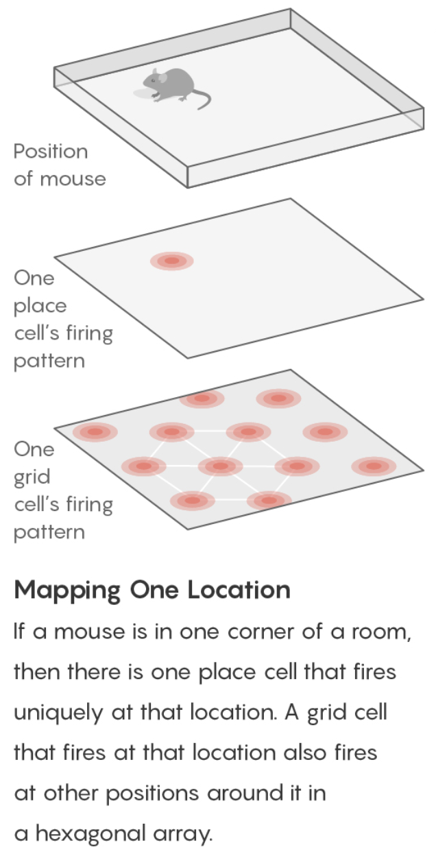
- navigation
- cognitive maps (tolman 1940s) - idea that rats in mazes learn spatial maps
- place cells (o’keefe 1971) - in the hippocampus - fire to indicate one’s current location
- remap to new locations
- grid cells (moser & moser 2005) - in the entorhinal cotex (provides inputs to the hippocampus) - not particular locations but rather hexagonal coordinate system
- grid cells fire if the mouse is in any location at the vertex (or center) of one of the hexagons
- there are grid cells with larger/smaller hexagons, different orientations, different offsets
- grid cells fire if the mouse is in any location at the vertex (or center) of one of the hexagons
- can look for grid cells signature in fmri: https://www.nature.com/articles/nature08704
- other places with grid cell-like behavior
- eye movement task
- some evidence for “time cells” like place cells for time
- sound frequency task https://www.nature.com/articles/nature21692
- 2d “bird space” task
1- introduction
1.1 - overview
- three types
- descriptive brain model - encode / decode external stimuli
- mechanistic brian cell / network model - simulate the behavior of a single neuron / network
- interpretive (or normative) brain model - why do brain circuits operate how they do
1.2 - descriptive
- receptive field - the things that make a neuron fire
1.3 - mechanistic and interpretive
- retina has on-center / off-surround cells - stimulated by points
- then, V1 has differently shaped receptive fields
- efficient coding hypothesis - learns different combinations (e.g. lines) that can efficiently represent images
- sparse coding (Olshausen and Field 1996)
- ICA (Bell and Sejnowski 1997)
- Predictive Coding (Rao and Ballard 1999)
- brain is trying to learn faithful and efficient representations of an animal’s natural environment
- same goes for auditory cortex
- brain is trying to learn faithful and efficient representations of an animal’s natural environment
2 - neural encoding
2.1 - defining neural code
- extracellular
- fMRI
- averaged over space
- slow, requires seconds
- EEG
- noisy
- averaged, but faster
- multielectrode array
- record from several individual neurons at once
- calcium imaging
- cells have calcium indicator that fluoresce when calcium enters a cell
- fMRI
- intracellular - can use patch electrodes
- raster plot
- replay a movie many times and record from retinal ganglion cells during movie
- encoding: P(response | stimulus)
- tuning curve - neuron’s response (ex. firing rate) as a function of stimulus
- orientation / color selective cells are distributed in organized fashion
- some neurons fire to a concept, like “Pamela Anderson”
- retina (simple) -> V1 (orientations) -> V4 (combinations) -> ?
- also massive feedback
- decoding: P(stimulus | response)
2.2 - simple encoding
- want P(response | stimulus)
- response := firing rate r(t)
- stimulus := s
-
simple linear model
- r(t) = c * s(t)
- weighted linear model - takes into account previous states weighted by f
- temporal filtering
- r(t) = $f_0 \cdot s_0 + … + f_t \cdot s_t = \sum s_{t-k} f_k$ where f weights stimulus over time
- could also make this an integral, yielding a convolution:
- r(t) = $\int_{-\infty}^t d\tau : s(t-\tau) f(\tau)$
- a linear system can be thought of as a system that searches for portions of the signal that resemble its filter f
- leaky integrator - sums its inputs with f decaying exponentially into the past
- flaws
- no negative firing rates
- no extremely high firing rates
- can add a nonlinear function g of the linear sum can fix this
- r(t) = $g(\int_{-\infty}^t d\tau : s(t-\tau) f(\tau))$
- spatial filtering
- r(x,y) = $\sum_{x’,y’} s_{x-x’,y-y’} f_{x’,y’}$ where f again is spatial weights that represent the spatial field
- could also write this as a convolution
- for a retinal center surround cell, f is positive for small $\Delta x$ and then negative for large $\Delta x$
- can be calculated as a narrow, large positive Gaussian + spread out negative Gaussian - can combine above to make spatiotemporal filtering - filtering = convolution = projection
- temporal filtering
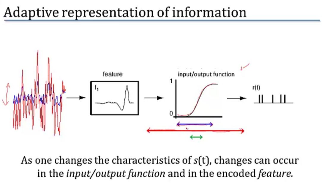
2.3 - feature selection
- P(response|stimulus) is very hard to get
- stimulus can be high-dimensional (e.g. video)
- stimulus can take on many values
- need to keep track of stimulus over time
- solution: sample P(response|s) to many stimuli to characterize what in input triggers responses
- find vector f that captures features that lead to spike
- dimensionality reduction - ex. discretize
- value at each time $t_i$ is new dimension
- commonly use Gaussian white noise
- time step sets cutoff of highest frequency present
- prior distribution - distribution of stimulus
- multivariate Gaussian - Gaussian in any dimension, or any linear combination of dimensions
- look at where spike-triggering points are and calculate spike-triggered average f of features that led to spike
- use this f as filter
- determining the nonlinear input/output function g
- replace stimulus in P(spike|stimulus) with P(spike|$s_1$), where s1 is our filtered stimulus
- use bayes rule $g=P(spike|s_1)=\frac{P(s_1|spike)P(spike)}{P(s_1)}$
- if $P(s_1|spike) \approx P(s_1)$ then response doesn’t seem to have to do with stimulus
- replace stimulus in P(spike|stimulus) with P(spike|$s_1$), where s1 is our filtered stimulus
- incorporating many features $f_1,…,f_n$
- here, each $f_i$ is a vector of weights
- $r(t) = g(f_1\cdot s,f_2 \cdot s,…,f_n \cdot s)$
- could use PCA - discovers low-dimensional structure in high-dimensional data
- each f represents a feature (maybe a curve over time) that fires the neuron
2.4 - variability
-
hidden assumptions about time-varying firing rate and single spikes
- smooth function RFT can miss some stimuli
-
statistics of stimulus can effect P(spike|stimulus)
- Gaussian white noise is nice because no way to filter it to get structure
- identifying good filter
- want $P(s_f|spike)$ to differ from $P(s_f)$ where $s_f$ is calculated via the filter
- instead of PCA, could look for f that directly maximizes this difference (Sharpee & Bialek, 2004)
- Kullback-Leibler divergence - calculates difference between 2 distributions
- $D_{KL}(P(s),Q(s)) = \int ds P(s) log_2 P(s) / Q(s)$
- maximizing KL divergence is equivalent to maximizing mutual info between spike and stimulus
- this is because we are looking for most informative feature
- this technique doesn’t require that our stimulus is white noise, so can use natural stimuli
- maximization isn’t guaranteed to uniquely converge
- modeling the noise
- need to go from r(t) -> spike times
- divide time T into n bins with p = probability of firing per bin
- over some chunk T, number of spikes follows binomial distribution (n, p)
- mean = np
- var = np(1-p)
- if n gets very large, binomial approximates Poisson
- $\lambda$ = spikes in some set time
- mean = $\lambda$
- var = $\lambda$
1. can test if distr is Poisson with Fano factor=mean/var=1
- interspike intervals have exponential distribution - if fires a lot, this can be bad assumption (due to refractory period)
- $\lambda$ = spikes in some set time
- generalized linear model adds explicit spike-generation / post-spike filter (Pillow et al. 2008)
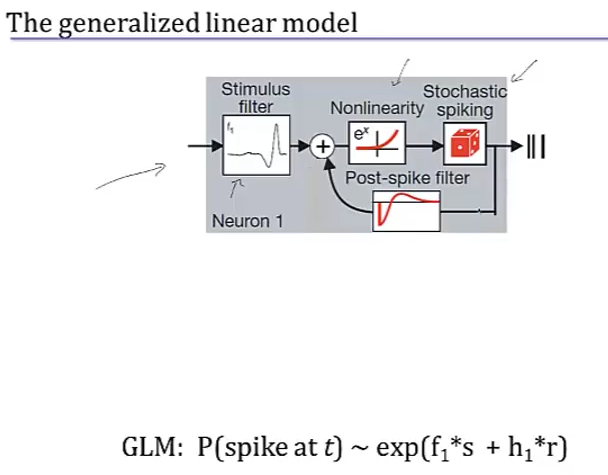
- post-spike filter models refractory period
- Paninski showed that using exponential nonlinearity allows this to be optimized
- could add in firing of other neurons
- time-rescaling theorem - tests how well we have captured influences on spiking (Brown et al 2001)
- scaled ISIs ($t_{i-1}-t_i$) r(t) should be exponential
3- neural decoding
3.1 - neural decoding and signal detection
- decoding: P(stimulus | response) - ex. you hear noise and want to tell what it is
- here r = response = firing rate
- monkey is trained to move eyes in same direction as dot pattern (Britten et al. 92)
- when dots all move in same direction (100% coherence), easy
- neuron recorded in MT - tracks dots
- count firing rate when monkey tracks in right direction
- count firing rate when monkey tracks in wrong direction
- as coherence decreases, these firing rates blur
- need to get P(+ or - | r)
- can set a threshold on r by maximizing likelihood
- P(r|+) and P(r|-) are likelihoods
- Neyman-Pearson lemma - likelihood ratio test is the most efficient statistic, in that is has the most power for a given size
- $\frac{p(r|+)}{p(r|-)} > 1?$
- can set a threshold on r by maximizing likelihood
- when dots all move in same direction (100% coherence), easy
- accumulated evidence - we can accumulate evidence over time by multiplying these probabilities
- instead we take sum the logs, and compare to 0
- $\sum_i ln \frac{p(r_i|+)}{p(r_i|-)} > 0?$
- once we hit some threshold for this sum, we can make a decision + or -
- experimental evidence (Kiani, Hanks, & Shadlen, Nat. Neurosci 2006)
- monkey is making decision about whether dots are moving left/right
- neuron firing rates increase over time, representing integrated evidence
- neuron always seems to stop at same firing rate
- priors - ex. tiger is much less likely then breeze
- scale P(+|r) by prior P(+)
- neuroscience ex. photoreceptor cells P(noise|r) is much larger than P(signal|r)
- therefore threshold on r is high to minimize total mistakes
- cost of acting/not acting
- loss for predicting + when it is -: $L_- \cdot P[+|r]$
- loss for predicting - when it is +: $L_+ \cdot P[-|r]$
- cut your losses: answer + when average Loss$+$ < Loss$-$
- i.e. $L_+ \cdot P[-|r]$ < $L_- \cdot P[+|r]$
- rewriting with Baye’s rule yields new test:
- $\frac{p(r|+)}{p(r|-)}> L_+ \cdot P[-] / L_- \cdot P[+]$
- here the loss term replaces the 1 in the Neyman-Pearson lemma
3.2 - population coding and bayesian estimation
- population vector - sums vectors for cells that point in different directions weighted by their firing rates
- ex. cricket cercal cells sense wind in different directions
- since neuron can’t have negative firing rate, need overcomplete basis so that can record wind in both directions along an axis
- can do the same thing for direction of arm movement in a neural prosthesis
- not general - some neurons aren’t tuned, are noisier
- not optimal - making use of all information in the stimulus/response distributions
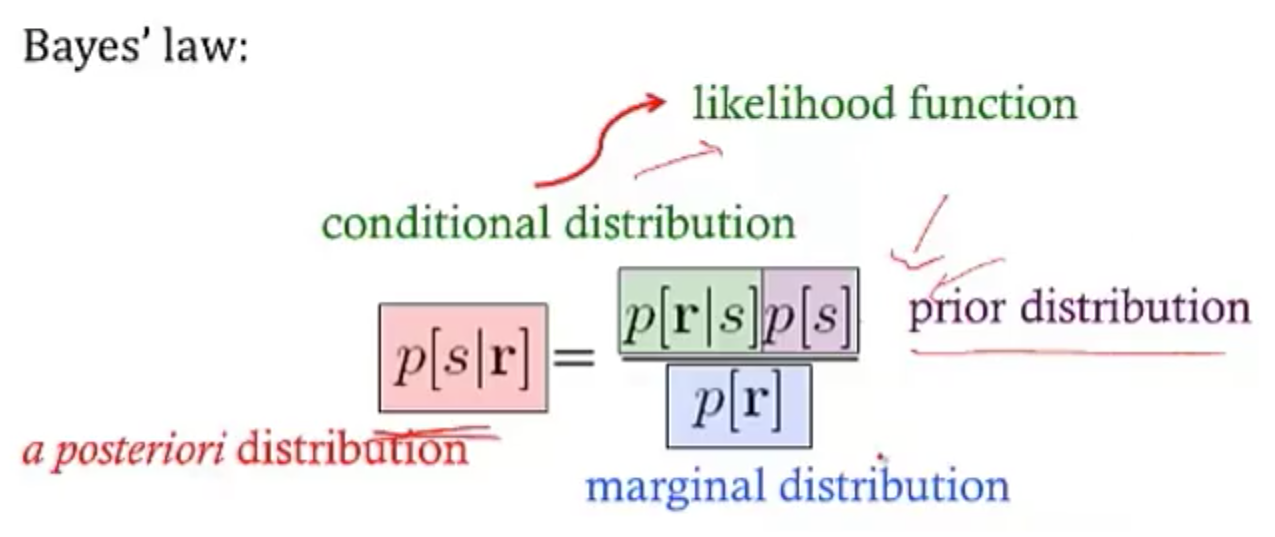
- bayesian inference
- $p(s|r) = \frac{p(r|s)p(s)}{p( r)}$
- maximum likelihood: s* which maximizes p(r|s)
- MAP = maximum $a:posteriori$: s* which mazimizes p(s|r)
- simple continuous stimulus example
- setup
- s - orientation of an edge
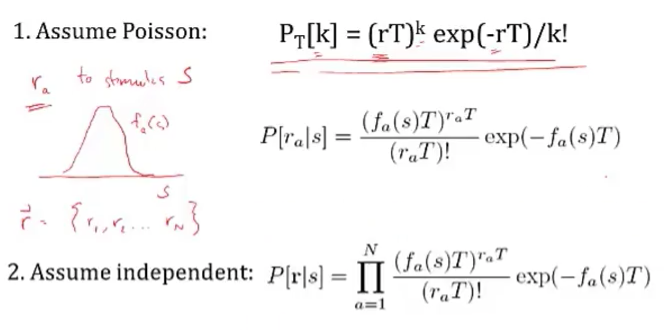
- each neuron’s average firing rate=tuning curve $f_a(s)$ is Gaussian (in s)
- let $r_a$ be number of spikes for neuron a
- assume receptive fields of neurons span s: $\sum r_a (s)$ is const
- solving
- maximizing log-likelihood with respect to s - take derivative and set to 0
- soln $s^* = \frac{\sum r_a s_a / \sigma_a^2}{\sum r_a / \sigma_a^2}$
- if all the $\sigma$ are same, $s^* = \frac{\sum r_a s_a}{\sum r_a}$
- this is the population vector
- maximum a posteriori
- $ln : p(s|r) = ln : P(r|s) + ln : p(s) = ln : P(r )$
- $s^* = \frac{T \sum r_a s_a / \sigma^2a + s{prior} / \sigma^2{prior}}{T \sum r_a / \sigma^2_a + 1/\sigma^2{prior}}$
- this takes into account the prior
- narrow prior makes it matter more
- doesn’t incorporate correlations in the population
- maximizing log-likelihood with respect to s - take derivative and set to 0
- setup
3.3 - stimulus reconstruction (not sure about this)
- decoding s -> $s^*$
- want an estimator $s_{Bayes}=s_B$ given some response r
- error function $L(s,s_{B})=(s-s_{B})^2$
- minimize $\int ds : L(s,s_{B}) : p(s|r)$ by taking derivative with respect to $s_B$
- $s_B = \int ds : p(s|r) : s$ - the conditional mean (spike-triggered average)
- add in spike-triggered average at each spike
- if spike-triggered average looks exponential, can never have smooth downwards stimulus
- could use 2 neurons (like in H1) and replay the second with negative sign
- LGN neurons can reconstruct a video, but with noise
- recreated 1 sec long movies - (Jack Gallant - Nishimoto et al. 2011, Current Biology)
- voxel-based encoding model samples ton of prior clips and predicts signal
- get p(r|s)
- pick best p(r|s) by comparing predicted signal to actual signal
- input is filtered to extract certain features
- filtered again to account for slow timescale of BOLD signal
- decoding
- maximize p(s|r) by maximizing p(r|s) p(s), and assume p(s) uniform
- 30 signals that have highest match to predicted signal are averaged
- yields pretty good pictures
- voxel-based encoding model samples ton of prior clips and predicts signal
4 - information theory
4.1 - information and entropy
- surprise for seeing a spike h(p) = $-log_2 (p)$
- entropy = average information
- code might not align spikes with what we are encoding
- how much of the variability in r is encoding s
- define q as en error
- $P(r_+|s=+)=1-q$
- $P(r_-|s=+)=q$
- similar for when s=-
- total entropy: $H(R ) = - P(r_+) log P(r_+) - P(r_-)log P(r_-)$
- noise entropy: $H(R|S=+) = -q log q - (1-q) log (1-q)$
- mutual info I(S;R) = $H(R ) - H(R|S) $ = total entropy - average noise entropy
- = $D_{KL} (P(R,S), P(R )P(S))$
- define q as en error
- grandma’s famous mutual info recipe
- for each s
- P(R|s) - take one stimulus and repeat many times (or run for a long time)
- H(R|s) - noise entropy
- $H(R|S)=\sum_s P(s) H(R|s)$
- $H(R ) $ calculated using $P(R ) = \sum_s P(s) P(R|s)$
- for each s
4.2 information in spike trains
- information in spike patterns
- divide pattern into time bins of 0 (no spike) and 1 (spike)
- binary words w with letter size $\Delta t$, length T (Reinagel & Reid 2000)
- can create histogram of each word
- can calculate entropy of word - look at distribution of words for just one stimulus
- distribution should be narrower - calculate $H_{noise}$ - average over time with random stimuli and calculate entropy
- varied parameters of word: length of bin (dt) and length of word (T)
- there’s some limit to dt at which information stops increasing
- this represents temporal resolution at which jitter doesn’t stop response from identifying info about the stimulus
- corrections for finite sample size (Panzeri, Nemenman,…)
- information in single spikes - how much info does single spike tell us about stimulus
- don’t have to know encoding, mutual info doesn’t care
- calculate entropy for random stimulus - $p=\bar{r} \Delta t$ where $\bar{r}$ is the mean firing rate
- calculate entropy for specific stimulus
- let $P(r=1|s) = r(t) \Delta t$
- let $P(r=0|s) = 1 - r(t) \Delta t$
- get r(t) by having simulus on for long time
- ergodicity - a time average is equivalent to averging over the s ensemble
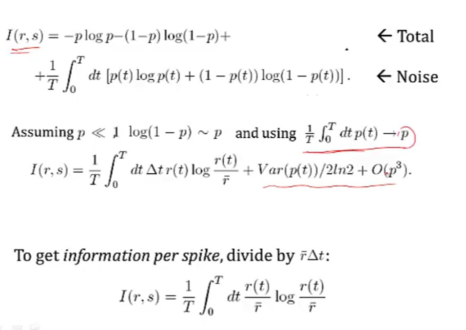
- info per spike $I(r,s) = \frac{1}{T} \int_0^T dt \frac{r(t)}{\bar{r}} log \frac{r(t)}{\bar{r}}$
- timing precision reduces r(t)
- low mean spike rate -> high info per spike
- ex. rat runs through place field and only fires when it’s in place field
- spikes can be sharper, more / less frequent
4.3 coding principles
- natural stimuli
- huge dynamic range - variations over many orders of magnitude (ex. brightness)
- power law scaling - structure at many scales (ex. far away things)
- efficient coding - in order to have maximum entropy output, a good encoder should match its outputs to the distribution of its inputs
- want to use each of our “symbols” (ex. different firing rates) equally often
- should assign equal areas of input stimulus PDF to each symbol
- adaptataion to stimulus statistics
- feature adaptation (Atick and Redlich)
- spatial filtering properties in retina / LGN change with varying light levels
- at low light levels surround becomes weaker
- coding sechemes
- redundancy reduction
- population code $P(R_1,R_2)$
- entropy $H(R_1,R_2) \leq H(R_1) + H(R_2)$ - being independent would maximize entropy
- correlations can be good
- error correction and robust coding
- correlations can help discrimination
- retina neurons are redundant (Berry, Chichilnisky)
- more recently, sparse coding
- penalize weights of basis functions
- instead, we get localized features
- redundancy reduction
- we ignored the behavioral feedback loop
5 - computing in carbon
5.1 - modeling neurons
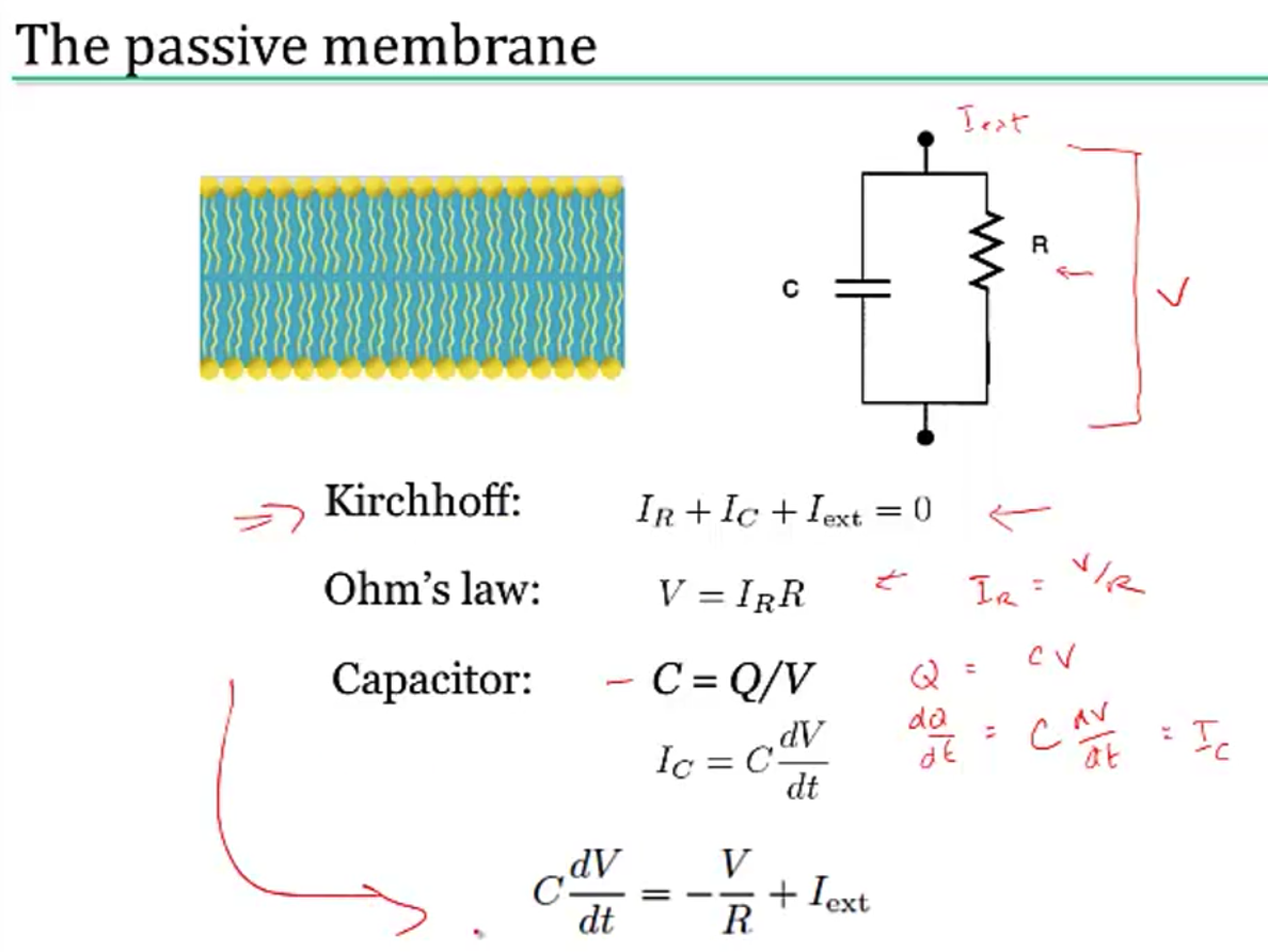
- nernst battery
- osmosis (for each ion)
- electrostatic forces (for each ion)
- together these yield Nernst potential $E = \frac{k_B T}{zq} ln \frac{[in]}{[out]}$
- T is temp
- q is ionic charge
- z is num charges
- part of voltage is accounted for by nernst battery $V_{rest}$
- yields $\tau \frac{dV}{dt} = -V + V_\infty$ where $\tau=R_mC_m=r_mc_m$
- equivalently, $\tau_m \frac{dV}{dt} = -((V-E_L) - g_s(t)(V-E_s) r_m) + I_e R_m $
- together these yield Nernst potential $E = \frac{k_B T}{zq} ln \frac{[in]}{[out]}$
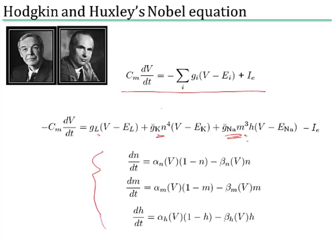
5.2 - spikes
5.3 - simplified model neurons
- integrate-and-fire neuron
- passive membrane (neuron charges)
- when V = V$_{thresh}$, a spike is fired
- then V = V$_{reset}$
- doesn’t have good modeling near threshold
- can include threshold by saying
- when V = V$_{max}$, a spike is fired
- then V = V$_{reset}$
- modeling multiple variables
- also model a K current
- can capture things like resonance
- theta neuron (Ermentrout and Kopell)
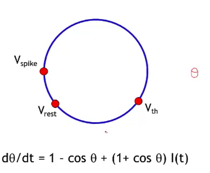
- often used for periodically firing neurons (it fires spontaneously)
5.4 - a forest of dendrites
- cable theory - Kelvin
- voltage V is a function of both x and t
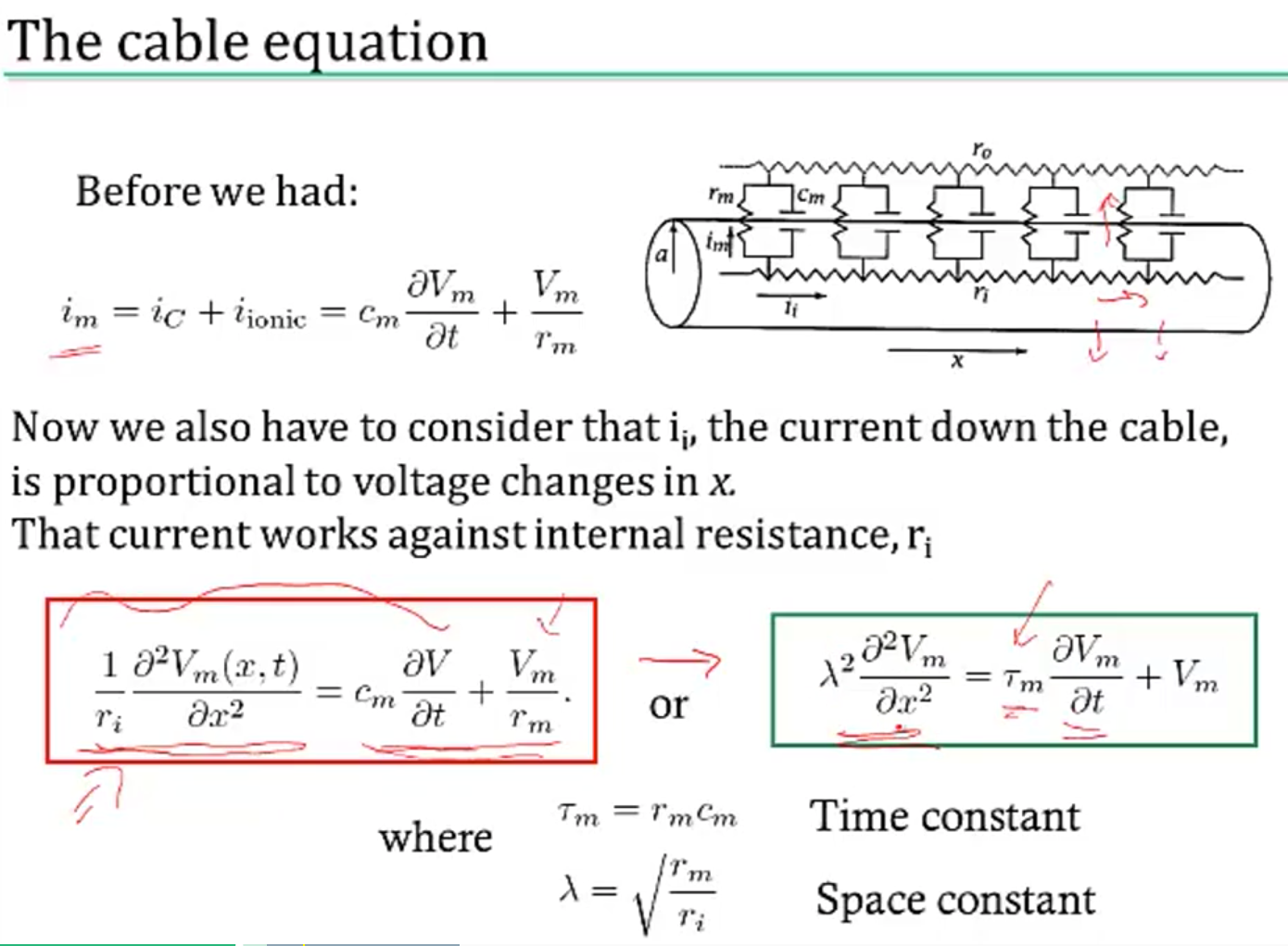
- separate into sections that don’t depend on x
- coupling conductances link the sections (based on area of compartments / branching)
- Rall model for dendrites
- if branches obey a certain branching ratio, can replace each pair of branches with a single cable segment with equivalent surface area and electrotonic length
- $d_1^{3/2} = d_{11}^{3/2} + d_{12}^{3/2}$
- if branches obey a certain branching ratio, can replace each pair of branches with a single cable segment with equivalent surface area and electrotonic length
- dendritic computation (London and Hausser 2005)
- hippocampus - when inputs arrive at soma, similiar shape no matter where they come in = synaptic scaling
- where inputs enter influences how they sum
- dendrites can generate spikes (usually calcium) / backpropagating spikes
- ex. Jeffress model - sound localized based on timing difference between ears
- ex. direction selectivity in retinal ganglion cells - if events arive at dendrite far -> close, all get to soma at same time and add
6 - computing with networks
6.1 - modeling connections between neurons
- model effects of synapse by using synaptic conductance $g_s$ with reversal potential $E_s$
- $g_s = g_{s,max} \cdot P_{rel} \cdot P_s$
- $P_{rel}$ - probability of release given an input spike
- $P_s$ - probability of postsynaptic channel opening = fraction of channels opened
- $g_s = g_{s,max} \cdot P_{rel} \cdot P_s$
- basic synapse model
- assume $P_{rel}=1$
- model $P_s$ with kinetic model
- open based on $\alpha_s$
- close based on $\beta_s$
- yields $\frac{dP_s}{dt} = \alpha_s (1-P_s) - \beta_s P_s$
- 3 synapse types
- AMPA - well-fit by exponential
- GAMA - fit by “alpha” function - has some delay
- NMDA - fit by “alpha” function - has some delay
- linear filter model of a synapse
- pick filter (ex. K(t) ~ exponential)
- $g_s = g_{s,max} \sum K(t-t_i)$
- network of integrate-and-fire neurons
- if 2 neurons inhibit each other, get synchrony (fire at the same time
6.2 - intro to network models
- comparing spiking models to firing-rate models
- advantages
- spike timing
- spike correlations / synchrony between neurons
- disadvantages
- computationally expensive
- uses linear filter model of a synapse
- advantages
- developing a firing-rate model
- replace spike train $\rho_1(t) \to u_1(t)$
- can’t make this replacement when there are correlations / synchrony?
- input current $I_s$: $\tau_s \frac{dI_s}{dt}=-I_s + \mathbf{w} \cdot \mathbf{u}$
- works only if we let K be exponential
- output firing rate: $\tau_r \frac{d\nu}{dt} = -\nu + F(I_s(t))$
- if synapses are fast ($\tau_s « \tau_r$)
- $\tau_r \frac{d\nu}{dt} = -\nu + F(\mathbf{w} \cdot \mathbf{u}))$
- if synapses are slow ($\tau_r « \tau_s$)
- $\nu = F(I_s(t))$
- if static inputs (input doesn’t change) - this is like artificial neural network, where F is sigmoid
- $\nu_{\infty} = F(\mathbf{w} \cdot \mathbf{u})$
- could make these all vectors to extend to multiple output neurons
- replace spike train $\rho_1(t) \to u_1(t)$
- recurrent networks
- $\tau \frac{d\mathbf{v}}{dt} = -\mathbf{v} + F(W\mathbf{u} + M \mathbf{v})$
- $-\mathbf{v}$ is decay
- $W\mathbf{u}$ is input
- $M \mathbf{v}$ is feedback
- with constant input, $v_{\infty} = W \mathbf{u}$
- ex. edge detectors
- V1 neurons are basically computing derivatives
- $\tau \frac{d\mathbf{v}}{dt} = -\mathbf{v} + F(W\mathbf{u} + M \mathbf{v})$
6.3 - recurrent networks
- linear recurrent network: $\tau \frac{d\mathbf{v}}{dt} = -\mathbf{v} + W\mathbf{u} + M \mathbf{v}$
- let $\mathbf{h} = W\mathbf{u}$
- want to investiage different M
- can solve eq for $\mathbf{v}$ using eigenvectors
- suppose M (NxN) is symmetric (connections are equal in both directions)
- $\to$ M has N orthogonal eigenvectors / eigenvalues
- let $e_i$ be the orthonormal eigenvectors
- output vector $\mathbf{v}(t) = \sum c_i (t) \mathbf{e_i}$
- allows us to get a closed-form solution for $c_i(t)$
- eigenvalues determine network stability
- if any $\lambda_i > 1, \mathbf{v}(t)$ explodes $\implies$ network is unstable
- otherwise stable and converges to steady-state value
- $\mathbf{v}_\infty = \sum \frac{h\cdot e_i}{1-\lambda_i} e_i$
- amplification of input projection by a factor of $\frac{1}{1-\lambda_i}$
- if any $\lambda_i > 1, \mathbf{v}(t)$ explodes $\implies$ network is unstable
- suppose M (NxN) is symmetric (connections are equal in both directions)
- ex. each output neuron codes for an angle between -180 to 180
- define M as cosine function of relative angle
- excitation nearby, inhibition further away
- memory in linear recurrent networks
- suppose $\lambda_1=1$ and all other $\lambda_i < 1$
- then $\tau \frac{dc_1}{dt} = h \cdot e_1$ - keeps memory of input
- ex. memory of eye position in medial vestibular nucleus (Seung et al. 2000)
- integrator neuron maintains persistent activity
- nonlinear recurrent networks: $\tau \frac{d\mathbf{v}}{dt} = -\mathbf{v} + F(\mathbf{h}+ M \mathbf{v})$
- ex. rectification linearity F(x) = max(0,x)
- ensures that firing rates never go below
- can have eigenvalues > 1 but stable due to rectification
- can perform selective “attention”
- network performs “winner-takes-all” input selection
- gain modulation - adding constant amount to input h multiplies the output
- also maintains memory
- ex. rectification linearity F(x) = max(0,x)
- non-symmetric recurrent networks
- ex. excitatory and inhibitory neurons
- linear stability analysis - find fixed points and take partial derivatives
- use eigenvalues to determine dynamics of the nonlinear network near a fixed point
7 - networks that learn: plasticity in the brain & learning
7.1 - synaptic plasticity, hebb’s rule, and statistical learning
- if 2 spikes keep firing at same time, get LTP - long-term potentiation
- if input fires, but not B then could get LTD - long-term depression
- Hebb rule $\tau_w \frac{d\mathbf{w}}{dt} = \mathbf{x}v$
- $\mathbf{x}$ - input
- $v$ - output
- translates to $\mathbf{w}_{i+1}=\mathbf{w}_i + \epsilon \cdot \mathbf{x}v$
- average effect of the rule is to change based on correlation matrix $\mathbf{x}^T\mathbf{x}$
- covariance rule: $\tau_w \frac{d\mathbf{w}}{dt} = \mathbf{x}(v-E[v])$
- includes LTD as well as LTP
- Oja’s rule: $\tau_w \frac{d\mathbf{w}}{dt} = \mathbf{x}v- \alpha v^2 \mathbf{w}$ where $\alpha>0$
- stability
- Hebb rule - derivative of w is always positive $\implies$ w grows without bound
- covariance rule - derivative of w is still always positive $\implies$ w grows without bound
- could add constraint that $||w||=1$ and normalize w after every step
- Oja’s rule - $||w|| = 1/\sqrt{alpha}$, so stable
- solving Hebb rule $\tau_w \frac{d\mathbf{w}}{dt} = Q w$ where Q represents correlation matrix
- write w(t) in terms of eigenvectors of Q
- lets us solve for $\mathbf{w}(t)=\sum_i c_i(0)exp(\lambda_i t / \tau_w) \mathbf{e}_i$
- when t is large, largest eigenvalue dominates
- hebbian learning implements PCA
- hebbian learning learns w aligned with principal eigenvector of input correlation matrix
- this is same as PCA
7.2 - intro to unsupervised learning
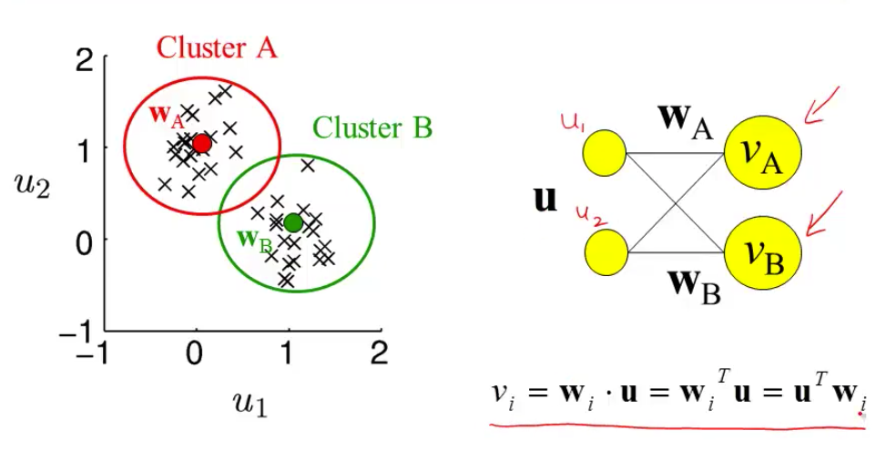
- most active neuron is the one whose w is closest to x
- competitive learning
- updating weights given a new input
- pick a cluster (corresponds to most active neuron)
- set weight vector for that cluster to running average of all inputs in that cluster
- $\Delta w = \epsilon \cdot (\mathbf{x} - \mathbf{w})$
- related to self-organizing maps = kohonen maps
- in self-organizing maps also update other neurons in the neighborhood of the winner
- update winner closer
- update neighbors to also be closer
- ex. V1 has orientation preference maps that do this
- updating weights given a new input
- generative model
- prior P(C )
- likelihoood P(X|C)
- posterior P(C|X)
- mixture of Gaussians model - Gaussian assumption P(X|C=c) is Gaussian
- EM = expectation-maximization
- estimate P(C|X) - pick what cluster point belongs to
- for Gaussian model, each cluster gets a probability of changing
- this probability weights the change - *“soft”
- learn parameters of generative model - change parameters of Gaussian (mean and variance) for clusters
- estimate P(C|X) - pick what cluster point belongs to
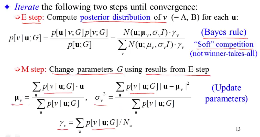
- assumes you have all the points at once
7.3 - sparse coding and predictive coding
- eigenface - Turk and Pentland 1991
- eigenvectors of the input covariance matrix are good features
- can represent images using sum of eigenvectors (orthonormal basis)
- suppose you use only first M principal eigenvectors
- then there is some noise
- can use this for compression
- not good for local components of an image (e.g. parts of face, local edges)
- if you assume Gausian noise, maximizing likelihood = minimizing squared error
- generative model
- images X
- causes
- likelihood P(X=x|C=c)
- Gaussian
- proportional to $exp(x-Gc)$
- want posterior P(C|X)
- prior p(C )
- assume priors causes are independent
- want sparse distribution
- has heavy tail (super-Gaussian distribution)
- then P(C ) = $k \cdot \prod exp(g(C_i))$
- can implement sparse coding in a recurrent neural network
- Olshausen & Field, 1996 - learns receptive fields in V1
- sparse coding is a special case of predicive coding
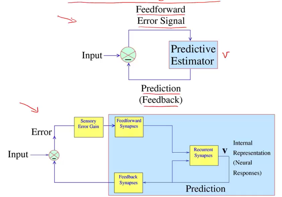
- there is usually a feedback connection for every feedforward connection (Rao & Ballard, 1999)
8.2 - reinforcement learning - predicting rewards
- dopamine serves as brain’s reward
ml analogies
Brain theories
- Computational Theory of Mind -Classical associationism -Connectionism -Situated cognition -Memory-prediction framework -Fractal Theory: https://www.youtube.com/watch?v=axaH4HFzA24 -Brain sheets are made of cortical columns (about .3mm diameter, 1000 neurons / column) -Have ~6 layers
brain as a computer
- Brain as a Computer – Analog VLSI and Neural Systems by Mead (VLSI – very large scale integration) -Brain Computer Analogy -Process info -Signals represented by potential -Signals are amplified = gain -Power supply -Knowledge is not stored in knowledge of the parts, but in their connections -Based on electrically charged entities interacting with energy barriers -http://en.wikipedia.org/wiki/Computational_theory_of_mind -http://scienceblogs.com/developingintelligence/2007/03/27/why-the-brain-is-not-like-a-co/ -Brain’ storage capacity is about 2.5 petabytes (Scientific American, 2005) -Electronics -Voltage can be thought of as water in a reservoir at a height -It can flow down, but the water will never reach above the initial voltage -A capacitor is like a tank that collects the water under the reservoir -The capacitance is the cross-sectional area of the tank -Capacitance – electrical charge required to raise the potential by 1 volt -Conductance = 1/ resistance = mho, siemens -We could also say the word is a computer with individuals being the processors – with all the wasted thoughts we have – the solution is probably to identify global problems and channel people’s focus towards working on them -Brain chip: http://www.research.ibm.com/articles/brain-chip.shtml -Differences: What Can AI Get from Neuroscience? -Brains are not digital -Brains don’t have a CPU -Memories are not separable from processing -Asynchronous and continuous -Details of brain substrate matter -Feedback and Circular Causality -Asking questions -Brains has lots of sensors -Lots of cellular diversity -NI uses lots of parallelism -Delays are part of the computation
Brain v. Deep Learning
- http://timdettmers.com/ -problems with brain simulations: -Not possible to test specific scientific hypotheses (compare this to the large hadron collider project with its perfectly defined hypotheses) -Does not simulate real brain processing (no firing connections, no biological interactions) -Does not give any insight into the functionality of brain processing (the meaning of the simulated activity is not assessed) -Neuron information processing parts -Dendritic spikes are like first layer of conv net -Neurons will typically have a genome that is different from the original genome that you were assigned to at birth. Neurons may have additional or fewer chromosomes and have sequences of information removed or added from certain chromosomes. -http://timdettmers.com/2015/03/26/convolution-deep-learning/ -The adult brain has 86 billion neurons, about 10 trillion synapse, and about 300 billion dendrites (tree-like structures with synapses on them