unsupervised
overview
- labels are not given
- intra-cluster distances are minimized, inter-cluster distances are maximized
- distance measures
- symmetric D(A,B)=D(B,A)
- self-similarity D(A,A)=0
- positivity separation D(A,B)=0 iff A=B
- triangular inequality D(A,B) <= D(A,C)+D(B,C)
- ex. Minkowski Metrics $d(x,y)=\sqrt[r]{\sum \vert x_i-y_i\vert ^r}$
- r=1 Manhattan distance
- r=1 when y is binary -> Hamming distance
- r=2 Euclidean
- r=$\infty$ “sup” distance
- correlation coefficient - unit independent
- edit distance
hierarchical
- two approaches:
- bottom-up agglomerative clustering - starts with each object in separate cluster then joins
- top-down divisive - starts with 1 cluster then separates
- ex. starting with each item in its own cluster, find best pair to merge into a new cluster
- repeatedly do this to make a tree (dendrogram)
- distances between clusters defined by linkage function
- single-link - closest members (long, skinny clusters)
- complete-link - furthest members (tight clusters)
- average - most widely used
- ex. MST - keep linking shortest link
- ultrametric distance - tighter than triangle inequality
- $d(x, y) \leq \max[d(x,z), d(y,z)]$
partitional
- partition n objects into a set of K clusters (must be specified)
- globally optimal: exhaustively enumerate all partitions
- minimize sum of squared distances from cluster centroid
- evaluation w/ labels - purity - ratio between dominant class in cluster and size of cluster
- k-means++ - better at not getting stuck in local minima
- randomly move centers apart
- Complexity: $O(n^2p)$ for first iteration and then can only get worse
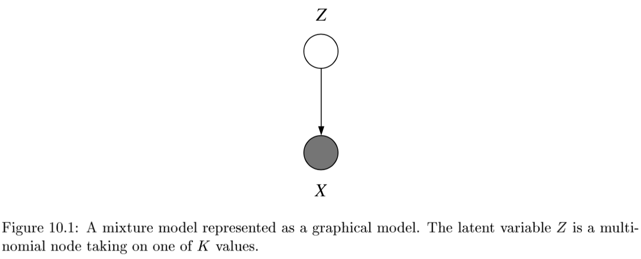
clustering (j 10)
- latent vars - values not specified in the observed data
-
- K-Means
- start with random centers
- E: assign everything to nearest center: $O(|\text{clusters}|*np) $
- M: recompute centers $O(np)$ and repeat until nothing changes
- partition amounts to Voronoi diagram
-
can be viewed as minimizing distortion measure $J=\sum_n \sum_i z_n^i x_n - \mu_i ^2$
-
GMMs: $p(x \theta) = \underset{i}{\Sigma} \pi_i \mathcal{N}(x \mu_i, \Sigma_i)$ -
$l(\theta x) = \sum_n \log : p(x_n \theta) \ = \sum_n \log \sum_i \pi_i \mathcal{N}(x_n \mu_i, \Sigma_i)$ -
hard to maximize bcause log acts on a sum
- “soft” version of K-means - update means as weighted sums of data instead of just normal mean
- sometimes initialize K-means w/ GMMs
-
conditional mixture models - regression/classification (j 10)
graph LR;
  X-->Y;
  X --> Z
  Z --> Y
- ex.
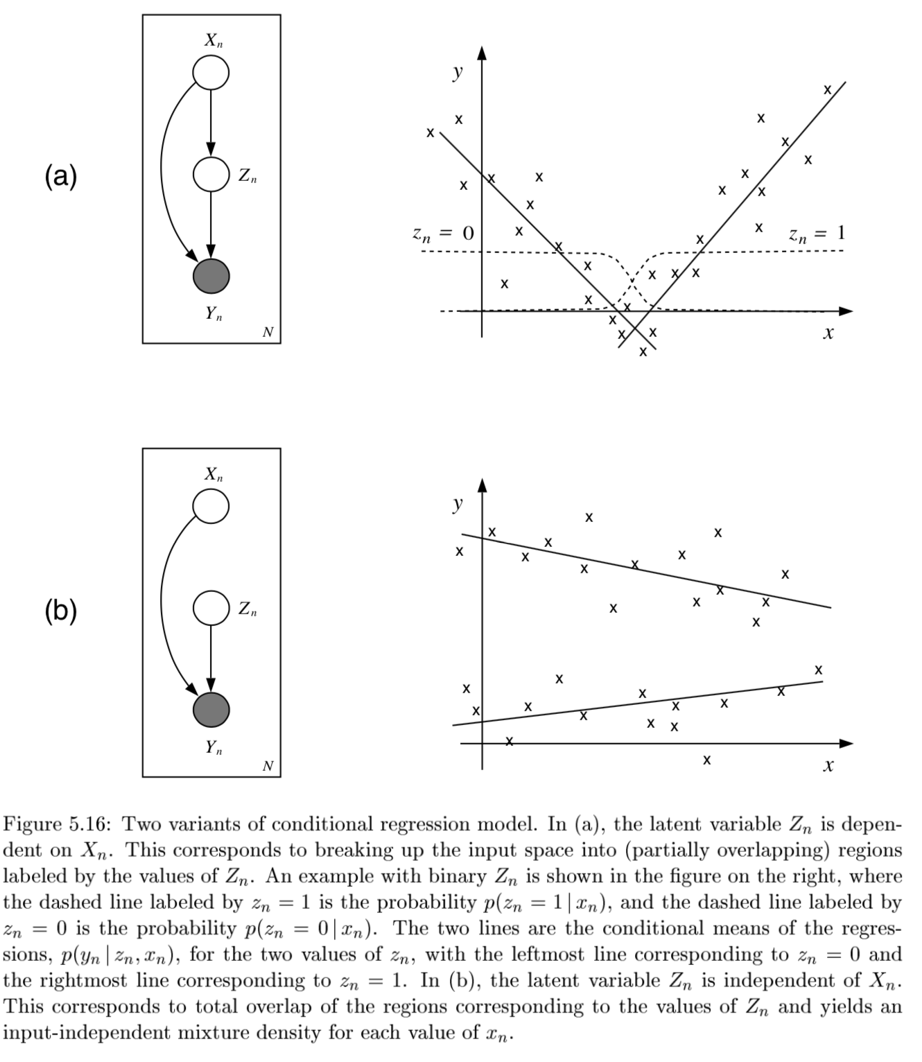
- latent variable Z has multinomial distr.
-
mixing proportions: $P(Z^i=1 x, \xi)$ - ex. $ \frac{e^{\xi_i^Tx}}{\sum_je^{\xi_j^Tx}}$
-
mixture components: $p(y Z^i=1, x, \theta_i)$ ~ different choices - ex. mixture of linear regressions
-
$p(y x, \theta) = \sum_i \underbrace{\pi_i (x, \xi)}_{\text{mixing prop.}} \cdot \underbrace{\mathcal{N}(y \beta_i^Tx, \sigma_i^2)}_{\text{mixture comp.}}$
-
- ex. mixtures of logistic regressions
-
$p(y x, \theta_i) = \underbrace{\pi_i (x, \xi)}{\text{mixing prop.}} \cdot \underbrace{\mu(\theta_i^Tx)^y\cdot[1-\mu(\theta_i^Tx)]^{1-y}}{\text{mixture comp.}}$ where $\mu$ is the logistic function
-
-
- also, nonlinear optimization for this (including EM)
spectral clustering
- use the spectrum (eigenvalues) of the similarity matrix of the data to perform dim. reduction before clustering in fewer dimensions
generative models
- overview: https://blog.openai.com/generative-models/
vaes
- just an autoencoder where the middle hidden layer is supposed to be unit gaussian
- add a kl loss to measure how well it maches a unit gaussian
- for calculation purposes, encoder actually produces means / vars of gaussians in hidden layer rather than the continuous values….
- this kl loss is not too complicated…https://web.stanford.edu/class/cs294a/sparseAutoencoder.pdf
- add a kl loss to measure how well it maches a unit gaussian
- generally less sharp than GANs
- uses mse loss instead of gan loss…
- intuition: vaes put mass between modes while GANs push mass towards modes
- constraint forces the encoder to be very efficient, creating information-rich latent variables. This improves generalization, so latent variables that we either randomly generated, or we got from encoding non-training images, will produce a nicer result when decoded.
gans
- train network to be loss function
autoregressive models
- model input based on input