optimization

• convex optimization
  • convex sets (boyd 2)
    • geometry
  • convex funcs (boyd 3)
  • optimization problems (boyd 4)
  • optimization
  • convex optimization
  • linear optimization
  • quadratic optimization
  • geometric program
  • generalized inequality
• duality (boyd 5)
  • optimality conditions
  • thms of alternatives
• approx + fitting (boyd 6)
  • norm approx problem
  • least norm problem
  • regularized approximation
  • robust approximation
  • function fitting
• unconstrained minimization (boyd 9)
  • unconstrained problems
  • descent methods
  • gd method
  • steepest descent method
  • newton’s method
• basic algorithms
• expectation maximization - j 11
• nn optimization
  • why is it hard?
  • complicated is simpler

---

convex optimization

convex sets (boyd 2)

• affine set: $x_1, x_2 \in C, \theta \in \mathbb{R} \implies \theta x_1 + (1 - \theta) x_2 \in C$

  • affine hull: aff C = {$\sum \theta_i x_i

    x_i \in C, \sum \theta_i =1 $}

• convex set: $x_1, x_2 \in C, 0 \leq \theta \leq 1 \implies \theta x_1 + (1 - \theta) x_2 ​$

  • convex hull: conv C = {$\sum \theta_i x_i :

    x_i \in C, \theta_i \geq 0, \sum \theta_i = 1$}

• cone: $\theta \geq 0 \implies \theta x \in C​$
• operations that preserve convexity
  • intersection (finite intersection of half-spaces)
  • pointwise max of affine funcs
  • composition
  • affine
  • perspective
  • linar fractional = projective
• generalized inequalities:
  • proper cone K: convex, closed, pointed, solid
    • $x \preceq_K y \iff y-x \in K$
• separating hyperplane thm: C, D convex $C \cap D =\emptyset \implies \exists a \neq 0, b : s.t. \ a^Tx \leq b \forall x \in C, \a^Tx \geq b \forall x \in D$

• supporting hyperplane thm: {$x

  a^tx = a^t x_0$} where $x_0$ on boundary of convex C

• dual cone $K^*$ = {$y

  x^Ty \geq 0 : \forall x \in K$}

  • $\preceq_{K^*}$ is dual of $\preceq_K$
  • $x \preceq_K y \iff \lambda^T x \leq \lambda^T y \quad \forall : \lambda \succeq_{K^*} 0$

geometry

• ellipsoid: {$x \in \mathbb{R}^n

  (x-x_c)^T P^{-1} (x-x_c) \leq 1$} where P symmetric, PSD

  • {$x_c + Au

    u

    _2 \leq 1$}

• hyperplane: {$x

  a^Tx = b$} ~ creates a halfspace

• norm cone: {$(x, t)

  :

  x

  \leq t$}

• polyhedron: {x

  Ax=b, Cx=d} = ${ \sum_i^k \theta_i v_i \;

  \sum_i^m \theta_i = 1, \theta_i \geq 0 } : m \leq k$

• simplex: conv{$v_{0:k}$}

convex funcs (boyd 3)

• definitions
  1. Jensen’s inequality $0 \leq \theta \leq 1$
     • $f(\theta x_1 + (1 - \theta) x_2) \leq \theta f(x_1) + (1 - \theta) f(x_2)$
     • $f(E[X]) \leq E[f(X)]$
  2. $\nabla^2 f(x) \succeq 0$
  3. $f(x_2) \geq f(x_1) + \nabla f(x_1)^T (x_2 - x_1)$
     • can show this by restricting to an arbitrary line
  4. consider epi f - also use things that preseve convexity
• concepts

  • epigraph epi f = ${ (x, t) \;

    : x \in dom f, f(x) \leq t }$

  • extended value extension: $\tilde{f}(x) = f(x)$ if $x \in dom f$ else $\infty$
  • wide sense function - can take on values $\pm \infty$

    • = dom f = {$x

      f(x) < \infty$}

  • wide sense convex func: $f(x) = inf { t \in \mathbb{R}

    (x, t) \in F}$ where $F \subseteq \mathbb{R}^{n+1}$

    • $F(x) = inf { t \in \mathbb{R}

      (x, t) \in F }$

  • $\alpha$-sublevel set of convex func is convex
• operations that preserve convexity
  • nonnegative weighted sums ~ multiplies for logs
  • affine map
  • pointwise max of convex
  • composition
  • perspective
  • minimization ~ sometimes
• conjugate of f
  • $f^*(y) = \underset{x \in dom f}{sup} : y^T x - f(x)$

  • dom $f^*$ = {$y

    f^*(y)$ is finite}

  • called Legendre transform when f differentiable
  • fenchel’s inequality: $f(x) + f^*(y) \geq x^ty$
  • $f^{**} = f$ iff convex, closed
• ex. $f(S) = log : det X^{-1}$
  • $f^*(Y) = \underset{X}{sup} [tr(YX) + log : det X]$
    • $= -n - log : det(-Y) $ if $-Y \in S^n_{++}$
• can use conj. to go other way: $f(y) = \underset{x}{sup}(y^Tx - f^*(x))$

optimization problems (boyd 4)

optimization

• standard form: $p^* = min : f_0(x)\s.t. : f_i(x) \leq 0 \ h_i(x) = 0$
• equivalent problems
  • change of vars
  • constraint transformations
  • slack vars
  • eliminating equalities
  • eliminating linear equalities
  • introducing equalities
  • optimizing over some vars ~ ex. quadratic
  • epigraph form: $min : t : s.t. : f_0 \leq t$
  • implicit + explicit constraints

convex optimization

• standard form: \(p^* = min \: f_0(x)\\s.t. \: f_i(x) \leq 0 \\ a_i^Tx = b_i\) where all f are convex
• optimality criteria (special cases of KKT)
  • x optimal if
    1. x is feasible
    2. $\nabla f_0 (x)^T(y-x) \geq 0 : \forall y $ feasible
  • if unconstrained $\nabla f_0 (x) = 0$
  • if equality only Ax=b, $\nabla f_0 (x) \perp N(A)$
  • $x \succeq 0$, $\nabla f_0 (x) \succeq 0; x_i (\nabla f_0 (x))_i = 0$
• equivalent convex problems
  • eliminating equality constraints
  • introducing equality constraints
  • slack vars ~ for linear inequalities
  • epigraph form
  • minimizing over some vars

linear optimization

• \[p^* = min \: c^T x + d\\s.t. \: Gx \succeq h \\ Ax=b\]
• standard form $x \succeq 0$ is the only inequality
• standard dual: max $-b^T \nu$ s.t. $A^T \nu + c \geq 0$
• linear-fractional program
  • $min : \frac{c^Tx + d}{e^tx+f} \ s.t : Gx \succeq h \ Ax = b$ ~ can be converted to LP

quadratic optimization

• \(min \: 1/2 x^TPx + q^Txr \\s.t. \: Gx \succeq h\) where $P \in S_+^n$
• QCQP - inequality constraints also convex

  • ex. $min :

    Ax-b

    _2^2$

• SOCP - $$min f^Tx \ s.t. :

  A_ix+b_i

  _2 \leq c_i^T + d_i \ Fx=g$$

geometric program

• \(min \: f_0(x) \\ s.t. \: f_i(x) \leq 1 \: i = 1:m \\ h_i(x) = 1 \: i = 1:p\) where $f_{0:m}$ posynomials, $h_i$ monomials
  • monomial $f(x) = c x_1^{a_1} \cdot x_n^{a_n}, c>0$
  • posynomial ~ sum of monomials ~ can transform into convex w/ $y_i = log x_i$

generalized inequality

• \[min \: f_0(x)\\s.t. \: f_i(x) \preceq_{K_i} 0, i=1:m\\Ax=b\]
• conic form problem: \(min \: c^Tx \\ s.t. \: Fx +g \preceq_K 0\\Ax=b\) ~ set $K=S_+^K$
• SDP = semi-definite program: \(min \: c^T x\\s.t. \: x_1F_1+...+x_nF_n+G \preceq 0\\Ax=b\) ~ where $F_1, …, F_n \in S^k$
  • standard form: $min : tr(CX) \ s.to : tr(A_iX)=b_i \ X \succeq 0$

duality (boyd 5)

• consider $\min : f_0 (x) \ s.t. : f_i(x) \leq 0 \ h_i(x) = 0$
• lagrangian $L(x, \lambda, \nu) = f_0(x) + \sum \lambda_i f_i(x) + \sum \nu_i h_i(x)$

• dual function $g(\lambda, \nu) = \underset{x \in D}{\inf} L(x, \lambda, \nu)$ ~ g always concave

  • $\lambda \succeq 0 \implies g(\lambda, \nu) \leq p^*$
• $(\lambda, \nu)$ dual feasible if
  1. $\lambda \succeq 0$
  2. $(\lambda, \nu) \in dom : g$
     • when $p^* = - \infty$, dual infeasible
     • when $d^*=\infty$, primal infeasible

• dual related to to conjugate func

  • ex. min f(x) s.t. $x = 0 \implies g(\nu) = -f^*(-\nu)$
• lagrange dual problem: $\max : g(\lambda, \nu)\s.t. : \lambda \succeq 0$

• weak duality: $d^* \leq p^*$

  • optimal duality gap: $p^* - d^*$
• strong duality: $d^* = p^*$ ~ requires more than convexity
• slater’s condition ~ if problem convex $\implies$ strong duality + $\exists$ dual optimal point
  • $\exists x \in relint : D\f_i(x) < 0\Ax = b$ ~ point is strictly feasible
  • to weaken this, affine $f_i$ can be $\leq 0$

• sion’s minimax thm: $x \to f(x, y)$ ~ conditions

  • $\implies \underset{x}{min} : \underset{y}{sup} : f(x,y) = \underset{y}{sup} : \underset{x}{min} : f(x,y)$

optimality conditions

• duality gap: $f_0(x) - g(\lambda, \nu)$
• can use stopping condition duality gap $\leq \epsilon_{abs}$ to be $\epsilon_{abs}$ - suboptimal
• strong duality yields complementary slackness
  • $\lambda_i f_i(x^*)=0$
• KKT optimality conditions ~ assume $f_0, f_i, h_i$ differentiable, strong duality
  1. $f_i(x^*) \leq 0$
  2. $h_i(x^*) = 0$
  3. $\lambda_i^* \geq 0$
  4. $\lambda_i^f(x_i^) = 0$
  5. $\nabla f_0 (x^) + \sum \lambda_i^ \nabla f_i (x_i^) + \sum \nu_i^ \nabla h_i (x^*) = 0$

thms of alternatives

• weak alternative - at most one of 2 is true
• strong alternative - exactly one is true
  • ex. Fredholm alternative
  • ex. Farkas’s lamma
    1. $\exists x : Ax \leq 0, c^Tx < 0$
    2. $\exists y : y \geq 0, A^Ty + c = 0$

approx + fitting (boyd 6)

norm approx problem

• minimize $

  Ax-b

  $

• ex. weighted norm approx. min

  W(Ax-b)

• ex. least squares min

  Ax-b

  $_2^2$

• ex. chebyshev approx norm min

  Ax-b

  $_\infty$

• ex. penalty function approx problem: $min : \phi(r_1) + … + \phi(r_m)\s.t. : r=Ax-b$

least norm problem

• min $

  x

  \s.t. : Ax=b$ ~ min $

  x_0+ Zu

  $, Z cols basis for N(A)

regularized approximation

• min $

  Ax-b

  + \gamma

  x

  $

• min $

  Ax-b

  ^2 + \gamma

  x

  ^2$

• Tikhonov: $min :

  Ax-b

  _2^2 + \gamma

  x

  _2^2$

• examples

  • ex. regularize w/

    Dx

  • ex. lasso
  • ex. quadratic smoothing
  • ex. total variation

robust approximation

• $A = \bar{A} + U$ ~ random w/ mean 0

  1. stochastic robust approx problem: $min : E

     Ax-b

     $

  2. (worst-case) robust approx prob: $min : sup

     Ax-b

     :

     A \in \mathcal{A}$

function fitting

• $f(u) = x_1 f_1 (u) + …. + x_n f_n (u)$ ~ $f_i$ are basis funcs, $x_i$ are coefficients
• sparse descriptions + basis pursuit
• interpolation

unconstrained minimization (boyd 9)

unconstrained problems

• $x^* = \text{argmin} : f(x) \implies \nabla f(x^*) = 0$
• examples
  • ex. quadratic: $\min : 1/2 x^TPX + q^Tx + r$
    • solved w/ $Px^* + q = 0$, if $P \succeq 0$, unique soln $-P^{-1}q$
  • ex. unconstrained geometric program
  • ex. analytic center of linear inequalities

    • $\min : f(x) = -\sum : \log (b_i - a_i^Tx)$ where dom f = ${x

      a_i^Tx< b_i, i = 1:m}$

• 3 definitions of convexity
  • $0 \leq \theta \leq 1$
    • $f(\theta x_1 + (1 - \theta) x_2) \leq \theta f(x_1) + (1 - \theta) f(x_2)$
  • $\nabla^2 f(x) \succeq 0$
  • $f(x_2) \geq f(x_1) + \nabla f(x_1)^T (x_2 - x_1)$
• $\color{red}0 \preceq \color{green}{\underset{\text{strong convexity}}{mI}} \preceq \nabla^2 \color{cornflowerblue}{f(x)} \preceq \underset{\text{smoothness}}{MI}$
  • $\kappa = M/m$ bounds condition number of $\nabla^2 f = \frac{\lambda_{\max}(\nabla^2 f)}{\lambda_{\min}(\nabla^2 f)}$
  • strongly convex: $\nabla^2 f(x) \succeq mI$

    • $\implies f(x_2) \geq f(x_1) + \nabla f(x_1)^T(x_2-x_1) + m/2

      x_2-x_1

      _2^2$

    • minimizing yields $p^* \geq f(x) - 1/(2m)

      \nabla f(x)

      _2^2$

    • if the gradient of f at x is small enough, then the difference between f(x) and p⋆ is small
  • smooth: $\exists : M, : \nabla^2f(x) \preceq MI$

    • $\implies f(y) \leq f(x) + \nabla f(x)^T(y-x) + M/2

      y-x

      _2^2$

• cond(C) = $W_{\max}^2 / W_{\min}^2​$

  • width of convex set $C \subset \mathbb{R}^n$ in direction q with $

    q

    _2=1$

  • $W(C, q) = \underset{z \in C}{\sup} : q^Tz - \underset{z \in C}{\inf} : q^Tz$

• alpha-level subset: $C_\alpha = {x

  f(x) \leq \alpha}$

descent methods

• update rule $x = x + t \Delta x$
• exact line search: $t = \underset{s \geq 0}{\text{argmin}} :f(x+s \Delta x)$
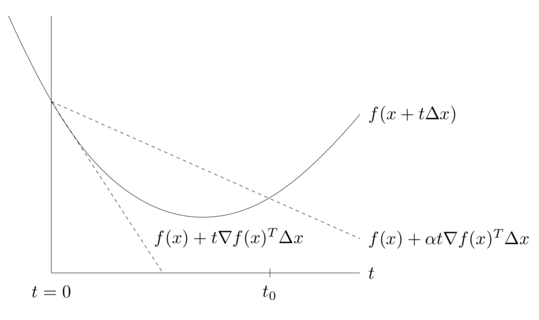
• backtracking line search
  • given a descent direction $\Delta x \text{ for } f, x \in dom : f, \alpha \in (0, 0.5), \beta \in (0, 1)$
  • t:=1, $\alpha \in (0, 0.5), \beta \in (0, 1)$
  • while $f(x + t \Delta x) > f(x) + \alpha t \nabla f(x)^T \Delta x$
    • $t *= \beta$
  • 

gd method

• convergence
  • can bound number of iterations required to be less than $\epsilon$
• examples
  • a quadratic problem in $R^2$
  • non-quadratic problem in $R^2$
  • a problem in $R^{100}$
  • gradient method and condition number
• conclusions
  • gd often exhibits approximately linear convergence
  • convergence rate depends greatly on $cond (\nabla^2 f(x))$ or sublevel sets

steepest descent method

• examples
  • euclidean norm: $\Delta x_{sd} = - \nabla f(x)$

  • quadratic norm $

    z

    _P = (z^TPz)^{1/2} =

    P^{1/2}z

    2$ where $P \in S{++}^n$

    • $\Delta x_{sd} = -P^{-1} \nabla f(x)$
  • $\ell_1$ norm: $\Delta_{sd} = -\frac{\partial f(x)}{\partial x_i} e_i$

newton’s method

• Newton step $\Delta x_{nt} = - \nabla^2 f(x)^{-1} \nabla f(x)$
  • PSD $\implies \nabla f(x)^T \Delta x_{nt} = - \nabla f(x)^T \nabla^2 f(x)^{-1} \nabla f(x) < 0$
• Newton’s method
  1. compute the newton step $\Delta x_{nt}$ and decrement $\lambda^2 = \nabla f(x)^T \nabla^2 f(x)^{-1} \nabla f(x)$
  2. stopping criterion: quit if $\lambda^2 / 2 \leq \epsilon​$
  3. line search: choose step size t w/ backtracking line search
  4. update: $x += t \Delta x_{nt}$

basic algorithms

• types: batch (have full data) vs online

1. gradient descent = batch gradient descent
   • gradient - vector that points to direction of maximum increase
   • at every step, subtract gradient multiplied by learning rate: $x_k = x_{k-1} - \alpha \nabla_x F(x_{k-1})$
   • alpha = 0.05 seems to work
   • $J(\theta) = 1/2 (\theta ^T X^T X \theta - 2 \theta^T X^T y + y^T y)$
   • $\nabla_\theta J(\theta) = X^T X \theta - X^T Y$
     • = $\sum_i x_i (x_i^T - y_i)$
     • this represents residuals * examples
2. stochastic gradient descent
   • don’t use all training examples - approximates gradient
     • single-sample
     • mini-batch (usually better in offline case)
   • coordinate-descent algorithm
   • online algorithm - update theta while training data is changing
   • when to stop?
     • predetermined number of iterations
     • stop when improvement drops below a threshold
   • each pass of the whole data = 1 epoch
   • benefits
     1. less prone to getting stuck to shallow local minima
     2. don’t need huge ram
     3. faster
3. newton’s method for optimization
   • second-order optimization - requires 1st & 2nd derivatives
   • $\theta_{k+1} = \theta_k - H_K^{-1} g_k$
   • update with inverse of Hessian as alpha - this is an approximation to a taylor series
   • finding inverse of Hessian can be hard / expensive
4. ADMM - alternating direction method of multipliers (ADMM) is an algorithm that solves convex optimization problems by breaking them into smaller pieces, each of which are then easier to handle

expectation maximization - j 11

• method to maximize likelihood on model with observed X and hidden Z
  1. expectation step - values of unobserved latent variables are filled in
     • calculates prob of latent variables given observed variables and current param values
  2. maximization step - parameters are adjusted based on filled-in variables
• goal: maximize complete log-likelihood, but don’t know z

  • expected complete log-likelihood $E_{p’}[l(\theta; x,z)] = \sum_z p’(z

    x,\theta) \cdot \log : p(x,z

    \theta)$

    • p’ distribution is assignment to z vars

  • deriving auxilary function $\mathcal L(q, \theta, x) = \sum_z p’(z

    x) \log \frac{p(x,z

    \theta)}{p’(z

    x)}$ - lower bound for the log likelihood

  • $\begin{align} l(\theta; x) &= \log : p(x

    \theta) & \text{incomplete log-likelihood} \&= \log \sum_z p(x,z

    \theta) &\text{complete log-likelihood}\&= \log\sum_z p’(z

    x) \frac{p(x,z

    \theta)}{p’(z

    x)} &\text{multiplying by 1} \ &\geq \sum_z p’(z

    x) \log \frac{p(x,z

    \theta)}{p’(z

    x)} &\text{Jensen’s inequality}\&\triangleq \mathcal L (p’, \theta) \end{align}$

  • this removes dependence on z
• steps

  • E: $p’(z

    x, \theta) = \underset{p’}{\text{argmax}}: \mathcal L(p’,\theta, x)$

  • M: $\theta = \underset{\theta}{\text{argmax}} : \mathcal L(p’, \theta, x)$
  • equivalent to maximizing expected complete log-likelihood
  • stochastically converges to local minimum
• alternatively, can look at kl-divergences

nn optimization

why is it hard?

• plateaus
• winding canyons
• cliffs
• local maxima to dodge
• saddle points (local max and local min)
• most popular
  • sgd
  • sgd + nesterov momentum
  • adam
  • adagrad - maintains a per-parameter learning rate that improves performance on problems with sparse gradients
  • rmsprop - (ignore) per-parameter learning rates that are adapted based on the average of recent magnitudes of the gradients for the weight (e.g. how quickly it is changing)
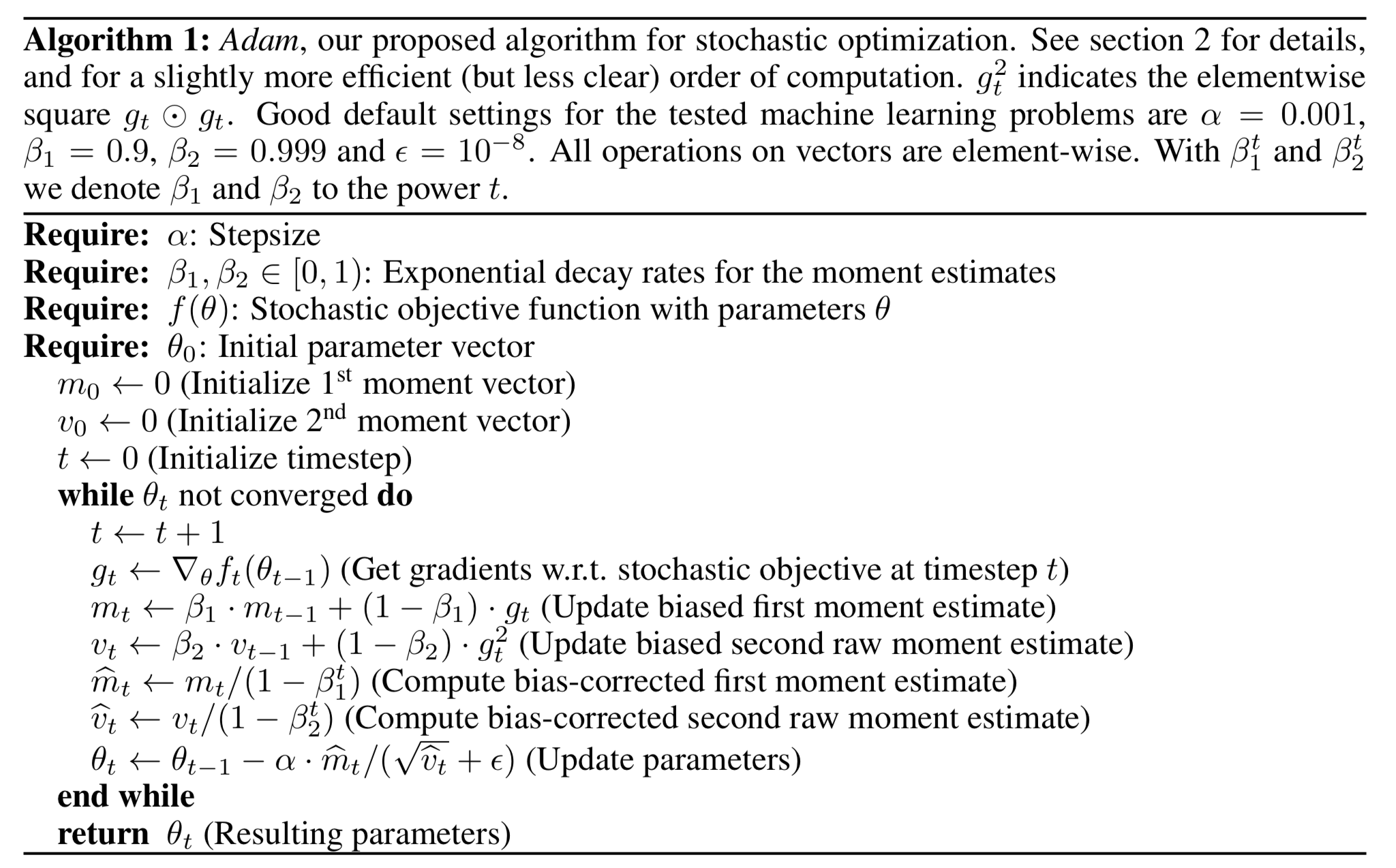
• adam - “adaptive moment estimation” (kingma_2015)
  • keep track of per-parameter learning rate (based on first moment of gradients tracked) and per-parameter second moment (based on variance of gradients tracked)
  • alpha - learning rate
  • beta1 - exponential decay rate for first moment estimate
    • default 0.9
  • beta2 - exponential decay rate for 2nd moment estimates (should be higher when gradients sparser)
    • default 0.999
  • epsilon - small number to prevent division by zero
    • default 1e-8 - usually requires tuning (ex. inception requires 1e-1) visualization
• requires low dims
  • goodfellow 2015 “Qualitatively characterizing neural network optimization problems” plots loss on line from starting point to ending point
  • could do PCA on params

complicated is simpler

• ex. $x^3 \sin(x)$ is simpler than just $x$ on the domain [−0.01, 0.01]
• dropout is like ridge